Physics problem: long stick floating on a liquid surface

The following problem, as many others, is coming from my usual source of inspiration, i.e. from Savchenko et al (1981) book. I am currently working through the section on surface tension phenomena. I decided to share this problem here mostly because of the beautiful answer, which is independent of surface tension coefficient of the liquid and of the stick's size, the result is just a number. Another reason for this post is that the problem is completely removed from newer editions of the book.

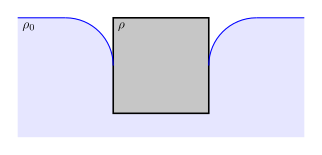
I did not pay much attention to the plot in the problem statement which is supposed to be used to get information necessary for the solution. I only realized that after Google AI turned my attention to the profile of the surface of the liquid prior to touching long sides of the stick.

Here is the translation of the problem statement:

A very long and thin stick with a square cross-section floats on the surface of a liquid, as shown in the figure. How much higher is the stick's density than the liquid's density (expressed as a ratio)?

We denote the length of the stick as $l$ and the side of its rectangular cross-section as $a$.

Let's consider forces acting on the stick along the vertical axis. Surface tension, buoyancy force and gravity, respectively, will compensate each other as follows:

\begin{align*} 2\sigma (l+a) + \rho_0 l a^2 g - \rho l a^2 g = 0 \end{align*}

where $\sigma$ is the surface tension coefficient, $\rho$ and $\rho_0$ are densities of the stick and of the liquid respectively.

The stick being very long and thin, means $l \gg a$ and we get the above equation simplified to:

\begin{align} 2\sigma + \rho_0 a^2 g - \rho a^2 g = 0 \end{align}

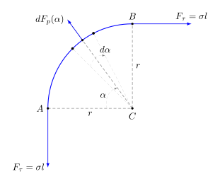
Now we consider the part of the liquid surface between the point where it touches the stick and the undisturbed horizontal plane. Let's denote this part of the liquid surface as $AB$ (see the figure). Now we approximate the form of $AB$ as a segment of a circle of radius $r$ (we will later take it to be $r=a/2$ as can be seen from the figure in the problem statement).

Let's consider horizontal forces acting on $AB$: $F_{px}$ - pressure force pushing the liquid towards the stick and $F_{\tau}$ surface tension preventing the liquid from touching the stick.

\begin{align*} F_x = F_{\tau} - F_{px} = 0 \end{align*}

$F_{\tau} = \sigma l$ - is the surface tension force applied at point $B$.

$F_p$ - is the total pressure force acting along the $AB$ parallel to the radius at each given point of $AB$. Its horizontal component is the following integral:

\begin{align*} F_{px} & = \int\limits_{0}^{\pi/2} dF_p(\alpha) \cos\alpha \\ & = \int\limits_{0}^{\pi/2} \rho_0 g l r(1-\sin\alpha) \cos\alpha \cdot r d \alpha = \\ & = \int\limits_{0}^{1} \rho_0 g l r^{2}(1-z) d z = \\ & = \frac{1}{2} \rho_0 g l r^{2} \end{align*}

Now the force balance equation gives us:

\begin{align*} & \sigma l - \frac{1}{2} \rho_0 g l r^{2} = 0 & \Rightarrow \\ & \sigma = \frac{\rho_0 g r^2}{2} & \end{align*}

Now, since $r = a/2$, we get

\begin{align*} \sigma = \frac{\rho_0 g a^2}{8} \end{align*}

Now we can use this expression for $\sigma$ in the equation obtained from the balance of the forces acting on the stick.

\begin{align*} & 2\sigma + \rho_0 a^2 g - \rho a^2 g = 0 & \Rightarrow \\ & \frac{\rho_0 g a^2}{4} + \rho_0 a^2 g - \rho a^2 g = 0 & \Rightarrow \\ & \frac{5}{4} \rho_0 - \rho = 0 & \Rightarrow \\ & \boxed{\frac{\rho}{\rho_0} = \frac{5}{4}} & \end{align*}

Finally the density of the stick is 1.25 times higher than the density of the liquid, and it still floats.

Zero-flow ocean boundary condition at the land-ocean interface

Recently, I was reading NEMO (Nucleus for European Modelling of the Ocean) manual, trying to fill in some blanks, as part of my professional development time. In the early pages, as it often happens to me, I got curious about the ocean-land boundary condition imposed on the ocean near its bottom, where water is limited by the land. In the manual it was given without derivation as:

$$ w = -(\vec{U}_h, \nabla_h H(x, y)) $$

where $\vec{U}_h$ - is the horizontal component of the ocean velocity, and $w$ - is the vertical component of the ocean velocity, $H(x, y)$ - is the ocean depth (aka bathymetry) at a point with coordinates $(x, y)$.

Below is the derivation, I've managed to come up with for this formula.

For each point on the surface $z=-H(x, y)$ we have a radius vector pointing from the origin of the coordinate system to any given point on $H(x, y)$ let's denote the radius vector as $\vec{r} = \vec{r}\left(x, y, z\right)$.

Let's also note that the total (3D) velocity of the ocean is $\vec{v} = \vec{U}_h + w \vec{k}$.

Where $\vec{k}$ is the unit vector (i.e $\left(\vec{k}, \vec{k}\right) = \left|\vec{k}\right|^2 = 1$) parallel to the vertical $z$-axis. Note that here our vertical axis is pointing upward, to be consistent with NEMO documentation.

Now the zero-flow condition through the ocean-land interface means that the projection of the total ocean velocity on the normal to the interface surface is 0:

$$ (\vec{v}, \vec{n}) = 0 $$

To find the expression for $\vec{n}$ we can use a vector product of $\partial_x \vec{r}$ and $\partial_y \vec{r}$, as these are tangent to $H(x,y)$ along the $x$ and $y$ axis respectively. Therefore,

$$ \vec{n}=[\partial_x \vec{r}, \partial_y \vec{r}] $$

we can expand the vector product as follows, using a determinant of the matrix below:

\begin{split} & \vec{n} & \; = \;&\begin{vmatrix} \vec{i} & \vec{j} & \vec{k} \\ 1 & 0 & -\partial_x H(x, y) \\ 0 & 1 & -\partial_y H(x, y) \end{vmatrix} = \vec{i}\, \partial_x H(x, y) + \vec{j}\,\partial_y H(x, y) + \vec{k} =\\ \\ & & \; = \; & \nabla H (x, y) + \vec{k}\\ \end{split}

Now when we plug the expressions above for $\vec{v}$ and $\vec{n}$ into the scalar product $(\vec{v}, \vec{n})$ we get:

\begin{align*} (\vec{v}, \vec{n}) & = \left(\vec{U}_h + w \vec{k}, \nabla H (x, y) + \vec{k} \right) \\ & = \left(\vec{U}_h, \nabla H (x, y)\right) + \left(\vec{U}_h, \vec{k}\right) + \left(w \vec{k}, \nabla H (x, y)\right) + w \\ & = \left(\vec{U}_h, \nabla H (x, y)\right) + w = 0 \\ \end{align*}

Above we used $\left(\vec{U}_h, \vec{k}\right)=0$ and $\left(w \vec{k}, \nabla H (x, y)\right) = 0$, since the scalar products of perpendicular vectors is 0.

Therefore, finally we can write the desired boundary condition as follows:

$$ \boxed{ w = -\left(\vec{U}_h, \nabla H (x, y)\right) }. $$

Physics problem: viscous flow in a cylindrical pipe

This problem is related to the previous one, where we discussed a setup with a fluid flow between two horizontal plates. The solution method is very similar, with a difference that here we select a cylindrical element and consider forces acting on it.

Problem statement

A liquid is pumped from one container to another through a long pipe of radius $R$ and length $l$. Determine the flow velocity in the pipe as a function of distance to its axis (i.e. to the center of the pipe). Given that the pressure drop between the two ends of the pipe is $\Delta P$ and the dynamic viscosity of the liquid is $\eta$.

Problem statement is taken from Savchenko et al (1981) book and translated by the post author.

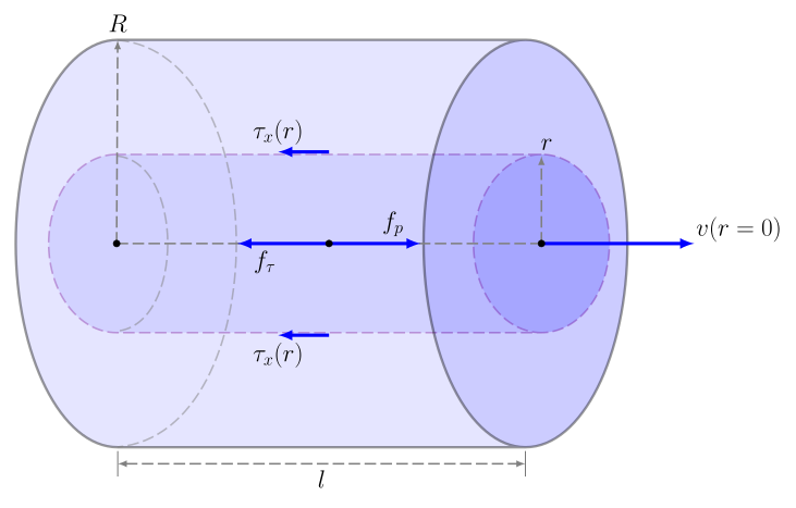
Exploiting the symmetry around the axis of the pipe we select a coaxial cylinder of radius $r$ in the flow and investigate forces acting on it.

Figure 1: Flow in pipe of length $l$ and radius $R$.

If we denote the viscosity stress along the cylinder's sides and parallel to its axis as $\tau_x(r)$, then we can write the balance of the viscous and pressure gradient forces acting on it, along the $x$-axis, as:

\begin{align*} & \tau_x(r) \cdot 2\pi r l + \Delta P \cdot \pi r^2 = 0 & \Rightarrow \\ & \tau_x(r) = -\frac{\Delta P r}{2 l} & \end{align*}

Now we can use the expression linking viscous stress and flow velocity gradient through the dynamic viscosity to determine the flow velocity as follows:

\begin{align*} & \tau_x(r) = -\frac{\Delta P r}{2 l} = \eta \frac{dv}{dr} & \Rightarrow \\ & \frac{dv}{dr} = -\frac{\Delta P r}{2 l \eta} & \Rightarrow \\ & \int\limits_{R}^{r} \frac{dv}{dr}\,dr = -\int\limits_{R}^{r}\frac{\Delta P r}{2 l \eta}\,dr & \Rightarrow \\ & v(r) - v(R) = -\frac{\Delta P \left( r^{2} - R^{2} \right) }{4 l \eta} \\ \end{align*}

Now using the non-slip condition at the pipe walls (i.e. $v(R) = 0$), we get the final expression for the flow velocity at a distance $r$ from the pipe axis: \begin{align*} \boxed{ v(r) = -\frac{\Delta P \left( r^{2} - R^{2} \right) }{4 l \eta} }. \end{align*}

Physics problem: viscous flow between two horizontal plates

Problem statement

Determine velocity of fluid in a stationary flow between two fixed horizontal plates as a function of position between the two plates. The distance between the plates is $h$ and the dynamic viscosity of the fluid is $\eta$. The pressure drop in the direction of the flow per unit length is $\frac{dP}{dx}=-\Delta P$. Additionally, compute the fluid discharge per unit of horizontal length perpendicular to the flow.

Problem statement is taken from Savchenko et al (1981) book and translated by the post author.

Solution

Tihs is not a praticularly complicated problem, but I find it important for understanding the momentum exchanges between layers of viscous fluids and it does not require very deep knowledge of the process but allows us to draw some interesting insights.

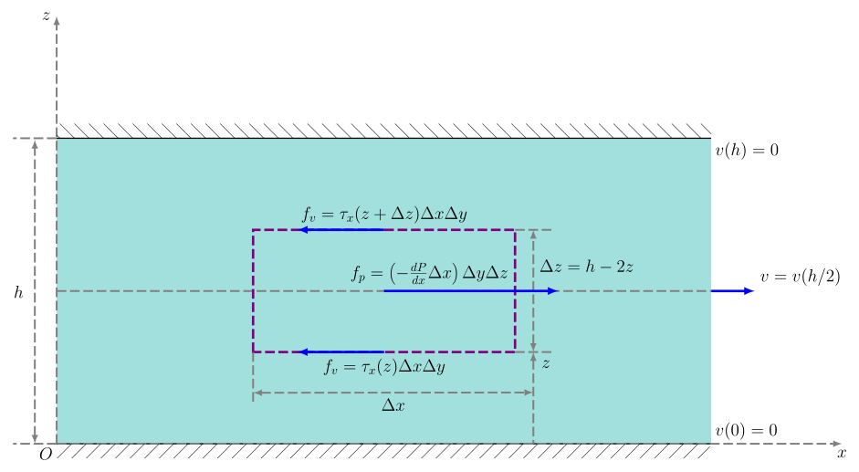
Let's introduce a coordinate system with $x$-axis along and pointing in the direction of flow, $z$-axis in the vertical direction upwards, and $y$-axis in the horizontal direction transversal to the flow and perpendicular to the plane formed by $x$ and $z$ axes. The origin of the coordinate system $O$ is on the lower plate (see Figure 1).

Figure 1: Vertical cross-section of the viscous flow between to horizontal plates. $y$-axis is perpendicular and points into the figure plane.

Since the flow is stationary and horizontally uniform the flow velocity is only a function of the vertical coordinate $z$: $v(z)$.

We assume a non-slip boundary condition near the horizontal plates: $v(z=0)=v(z=h)=0$. Additionally, we assume that the stress (friction force per unit of contact area between horizontal layers of the fluid, $\tau_x$) due to viscosity decreases towards the plane of symmetry of the flow: $z=h/2$, i.e the layers of the fluid closer to the middle have higher velocities. Therefore, we can determine $v(z)$ for $z \in [0, h/2]$ and then use the symmetry of the flow to find the velocity for $z \in [h/2, h]$.

Let's consider an element of fluid with dimensions $(\Delta x, \Delta y, \Delta z = h - 2z)$ with it's lower face at $z \in [0, h/2]$ and parallel to the axes $x$ and $y$. Assuming that the viscous stress $x$-coordinate $\tau_x(z)$ is negative, we can express the balance of the forces acting on the selected element of fluid along the $x$-axis as follows:

\begin{align*} \tau_x(z) \cdot \Delta x \cdot \Delta y + \tau_x(z + \Delta z) \cdot \Delta x \cdot \Delta y + \Delta P \cdot \Delta x \cdot \Delta y \cdot \Delta z = 0 \end{align*}

It is easy to see that with $\Delta z = h - 2z$ the upper and lower faces of the selected element are symmetric with respect to the middle plane of the flow ($z=h/2$), and are at the same distance from the upper and lower plates respectively (this is by design of our imaginary flow element) which means that $\tau_x(z + \Delta z) = \tau_x(z)$. Then we can simplify the above balance of forces as:

\begin{align*} & 2 \tau_x(z) + \Delta P \cdot \Delta z = 0 & \Rightarrow \\ & 2 \tau_x(z) + \Delta P \cdot (h - 2z) = 0 & \Rightarrow^{\,} \\ & \tau_x(z) = -\frac{\Delta P}{2} (h - 2z) & \end{align*}

The above expression for the stress is valid for $z \in [0, h/2]$.

Let's now determine $v(z)$ for $z \in [0, h/2]$ and then we'll use the symmetry of the flow to extend the solution to the whole range $z \in [0, h]$.

We can now use the relation between the velocity and the stress through the dynamic viscosity $\eta$:

\begin{align*} \tau_x(z) = -\eta\frac{dv}{dz}, \; z \in [0, h/2] \end{align*}

Using previously derived expression for $\tau_x(z)$ and then integrating we get:

\begin{align*} & -\frac{\Delta P}{2} (h - 2z) = -\eta\frac{dv}{dz} & \Rightarrow \\ & v(z) = \frac{\Delta P}{2\eta} \left( hz -z^{2} \right) + C & \end{align*}

where $C$ is the constant of integration.

Then using the non-slip condition at the plates we determine the integration constant as $C = v(z=0)=0 \Rightarrow C=0$ and the final expression for the velocity profile is:

\begin{align*} v(z) = \frac{\Delta P}{2\eta} z (h - z), \; z \in [0, h/2]. \end{align*}

Now for $z \in [h/2, h]$ we can use the flow symmetry to express the flow velocity as:

\begin{align*} \hat{v}(z) = v(h - z) = \frac{\Delta P}{2\eta} (h - z) z, \; z \in [h/2, h]. \end{align*} which, curiously, is the same expression as for $z \in [0, h/2]$, therefore finally the flow velocity profile can be expressed using a single formula:

\begin{align*} \boxed{v(z) = \frac{\Delta P}{2\eta} (h - z) z, \; z \in [0, h]} \end{align*}

In the second part of the problem we are asked to compute the flux density per unit of length in $y$ direction, i.e. $q=\frac{dQ}{dy}$. This is just a simplification for us to use a simpler flux expression ($\int{v\,dz}$) instead of the more general one ($\iint{v\,dy\,dz}$).

Therefore we obtain the flux density by integrating the above profile:

\begin{align*} &q=\int\limits_{0}^{h}v(z)\,dz & \Rightarrow \\ &q=\int\limits_{0}^{h} \frac{\Delta P}{2\eta} (h - z) z \,dz &\Rightarrow \\ &q= \frac{\Delta P}{2\eta} \left(\frac{h^{3}}{2} - \frac{h^{3}}{3} \right) & \Rightarrow \\ &\boxed{q= \frac{\Delta P h^{3}}{12\eta}} & \end{align*}

Physics problem: Collapsing spherical cavity (bubble) in a water pond

Consider a collapsing spherical cavity in a large pond of water. The initial pressure of water in the pond is $P_0$, the initial radius of the cavity is $R_0$. Determine the speed of the edge of the cavity when its radius reaches $r_0$ ($r_0 < R_0$). The water density is $\rho$.

Note: The problem statement is translated (and slightly modified) from the original text in Savchenko et al 1981.

Discussion

I did not plan on writing up this problem as it seemed trivial to me at first. I thought, ok there is some kind of differential equation to compose and solve.

I tried to use the Newton's law and the energy conservation equation approaches but could not really get it.

I asked ChatGPT, and it came up with a solution based on the energy balance equation, the solution did resemble the correct one but it was off by a constant factor. ChatGPT mentioned the Rayleigh-Plesset equation which helped me to come up with my solution below. But here I decided to base the solution on the Newton's equation of motion to be able to present a self-contained solution, at least from my stand point.

Solution

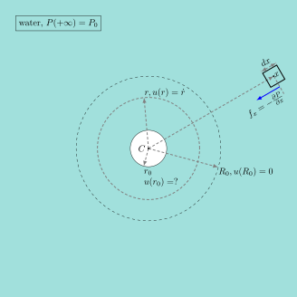
Let's consider a water parcel at a distance $x$ from the center of the cavity $C$ (see the figure below).

Figure 1: Cross-section of collapsing cavity in a large pond. Dashed circles show positions of the cavity's edge when its sizes are $R_0, r, r_0$.

The pressure gradient will act to accelerate the parcel towards the point $C$.

\begin{equation} \rho \frac{dv}{dt} = -\frac{\partial P}{\partial x} \end{equation}

where $v=v(x, t)$ - is velocity of the water parcel at the distance $x$ from the center of the collapsing hollow cavity at time $t$.

We can express the derivative of $v(x(t), t)$ in the above equation by assuming that the parcell travels along a tragectory $x(t)$ and employing the compound function differentiation formula:

\begin{align*} \frac{dv}{dt} &= \frac{\partial v}{\partial t} + \frac{\partial v}{\partial x} \frac{d x}{d t} \\ &= \frac{\partial v}{\partial t} + v\frac{\partial v}{\partial x} \end{align*}

Therefore, the equation of motion takes the following form (this is also known as an Euler form of the equation of motion): \begin{align} \boxed{\frac{\partial v}{\partial t} + v\frac{\partial v}{\partial x} = -\frac{1}{\rho}\frac{\partial P}{\partial x}} \end{align}

Let's consider the continuity equation for the spheres with radii $x$ and $R_0$ and centered around the point $C$:

\begin{align*} & v(x, t) \cdot 4\pi x^2 = v(R_0, t) \cdot 4\pi R_0^2 & \Rightarrow \\ & v(x, t) \cdot x^2 = v(R_0, t) \cdot R_0^2 = F(t) & \Rightarrow \\ & \boxed{v(x, t) = \frac{F(t)}{x^2}} & \end{align*}

Now let's plug the above expression for $v(x, t)$ into the equation of motion:

\begin{align*} & \frac{1}{x^2} \frac{d F(t)}{d t} + \frac{F(t)^2}{x^2}\left(-\frac{2}{x^3} \right) = -\frac{1}{\rho}\frac{\partial P}{\partial x} & \Rightarrow \\ & \frac{1}{x^2} \frac{d F(t)}{d t} - \frac{2F(t)^2}{x^5} = -\frac{1}{\rho}\frac{\partial P}{\partial x} \end{align*}

Let's consider the above equation at a fixed moment in time when the radius of the hollow cavity is $r(t)$. Then integrating the above equation from $r(t)$ to $+\infty$ and using that $P(r) = 0$ and $P(+\infty)=P_0$ we get:

\begin{align*} & \frac{d F(t)}{d t}\int\limits_r^{+\infty}\frac{dx}{x^2} - 2F(t)^2\int\limits_r^{+\infty}\frac{dx}{x^5} = -\frac{1}{\rho}\int\limits_r^{+\infty}\frac{\partial P}{\partial x} dx & \Rightarrow \\ & \frac{1}{r}\frac{d F(t)}{d t} - \frac{1}{2} \frac{F(t)^2}{r^4} = -\frac{P_0}{\rho} & \end{align*}

We can express $F(t)$ using flux continuity at the edge of the cavity as follows:

\begin{align*} F(t) = u(t)r^2 \end{align*}

where $u(t) = dr/dt=\dot{r}$ - is the speed of the edge of the cavity at time $t$ when its radius is $r=r(t)$.

After plugging in the above expression for $F(t)$ into the integrated equation of motion, we get:

\begin{align*} \boxed{\dot{u}r + \frac{3}{2} u^2 = -\frac{P_0}{\rho}} \end{align*}

The above is a particular case of an existing named equation (Rayleigh-Plesset equation: $\ddot{r} r + \frac{3}{2} \dot{r}^2 = -P_0/\rho$, where $\dot{r}=u$).

Finally, to solve the equation we will invert the $r(t)$ function and will consider the speed of the edge of the cavity as a function of the radius of the cavity.

\begin{align*} \dot{u} = \frac{d u}{d r} \frac{1}{\dot{r}} \end{align*}

Replacing the temporal derivative $\dot{u}$, using the above formula, in the initial differential equation we get an easily separable first order differential equation with respect to $u=u(r)$:

\begin{align*} \frac{du}{dr}ur + \frac{3}{2} u^2 = -\frac{P_0}{\rho} \end{align*}

Further, we can separate $du$ and $dr$ and integrate the equation from $R_0$ to $r_0$, taking into account that $u(R_0) = 0$ (i.e. the velocity of the cavity edge was 0 in the beginning when its radius was $R_0$):

\begin{align*} & -\int\limits_{u(R_0)}^{u(r_0)} \frac{u du}{\frac{P_0}{\rho} + \frac{3}{2}u^2} = \int\limits_{R_0}^{r_0}\frac{dr}{r} & \Rightarrow \\ & \ln\left(\frac{\frac{P_0}{\rho} + \frac{3}{2}u_(r_0)^2}{\frac{P_0}{\rho}}\right) = -3 \ln\left(\frac{r_0}{R_0}\right) & \Rightarrow \\ & \frac{P_0}{\rho} + \frac{3}{2}u(r_0)^2 = \frac{P_0}{\rho}\left(\frac{R_0}{r_0}\right)^3 & \Rightarrow \\ & \boxed{\left| u(r_0)\right| = \sqrt{\frac{2}{3}\frac{P_0}{\rho}\frac{R_0^3 - r_0^3}{r_0^3}} } & \end{align*}

So the above expression is the formula for the speed of the edge of the collapsing cavity at the moment when its radius reaches $r_0$ from $R_0$. It is interesting to note that there is a singularity at $r_0 \rightarrow 0$, the speed of the cavity edge increases to infinity.

Physics problem: acceleration of water level in a container due to draining from an opening in its bottom

Problem statement

From an opening at the bottom of a tall container, water drains out. The cross-section area of the container is $S$, and the cross-section area of the draining stream of water is $\sigma$. The water level in the vessel moves downward with constant acceleration. Determine this acceleration.

Solution

I'll describe two methods to solve the problem: the first one is the one I used and it is based on Bernoulli's law (energy conservation) and the second one is using the Toricelli's formula and accompanying assumptions from the get go. The second one I would guess a more experimented physicist would use and be done with it (see the approach 2). If I were to think about the second approach right away, this post would not happen.

Approach 1

Let's denote the speed of the water at the surface of the container and at the draining hole as $v_0$ and $v_1$ respectively. Then we can write energy and mass conservation expressions for the two cross-sections as follows:

\begin{align*} \begin{cases} \frac{v_0^2}{2} + gh = \frac{v_1^2}{2} \\ v_1\sigma = v_0 S \end{cases} \end{align*}

where $h$ is the current water level in the container, ang $g$ is the acceleration due to gravity.

Now, if we eliminate $v_1$ from the energy conservation equation and apply a time derivative to the both sides of the equation we will obtain the following relation (we use an upper dot to denote a time derivative, $\dot{x}=\frac{dx}{dt}$):

\begin{equation*} 2 v_0 \dot{v_0} + 2g\dot{h}=\left(\frac{S}{\sigma}\right)^2 2 v_0 \dot{v_0} \end{equation*}

Let's denote the acceleration of the water level as $a=\dot{v_0}$, and also note that $v_0 = -\dot{h}$ (the minus sign here is added because the level $h$ is decreasing with time and I prefer to consider $v_0$ as speed value without direction). Using this notation, the previous equation can be written as:

\begin{equation*} 2 v_0 a - 2gv_0=\left(\frac{S}{\sigma}\right)^2 2 v_0 a \end{equation*}

Simplifying we get the following expression for the water level acceleration in the container:

\begin{equation*} a = \frac{g}{1 - \left(\frac{S}{\sigma}\right)^2} \end{equation*}

Now we could consider that the conditions given in the problem statement imply $S\gg\sigma \rightarrow S/\sigma \gg 1$, therefore we can approximate the above expression as:

\begin{equation*} a \approx -g\left(\frac{\sigma}{S}\right)^2 \end{equation*}

Note that $a = \dot{v_0} < 0$, meaning that the water level descent in the container is slowing down with time.

Approach 2

For this approach we recognize right away that the problem conditions allow the use of Toricelli's formula for the speed $v_1$ of draining water from a large container with the water level at $h$:

\begin{equation*} v_1=\sqrt{2gh} \end{equation*}

The draining water will cause the change to the water level as follows: \begin{align*} \dot{h}=-v_1\sigma/S=-\frac{\sigma}{S}\sqrt{2gh} \end{align*}

If we apply a time derivative to the above equation and substitute $\dot{h}$, we obtain:

\begin{align*} \ddot{h} & =-\frac{\sigma}{S}\sqrt{2g}\frac{1}{2\sqrt{h}}\dot{h} \\ & = g\left(\frac{\sigma}{S}\right)^2 \end{align*}

Since the water level acceleration is $a = \dot{v_0} = d_t \left( -\dot{h} \right) = -\ddot{h}$, we obtain the final expression using the above relation for the second derivative of the water level as:

\begin{align*} a = -g\left(\frac{\sigma}{S}\right)^2 \end{align*}

Note that in this case we did not have to make any approximations as they were already applied for the Toricelli's formula to be valid (mainly that the speed of the water level $v_0$ is much lower than the draining speed $v_1$).

Physics problem: cumulative shell colliding with an armoured wall

Introduction and problem statement

This problem, as many others appearing here, took me a lot of time to wrap my head around. I almost lost faith, even tried to ask ChatGPT to solve it for me few times, but ChatGPT's solution was wrong or completely obscure for me.

Here is the problem statement (translated by ChatGPT from the Savchenko et al 1981 book).

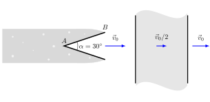
Problem statement: In 1941, the Germans invented a cumulative anti-tank shell. The shell has a fuse on its front part, which, upon impact, causes detonation and ignites the entire charge. The shell penetrates the armor. In 1944, such German shells came into the hands of both the Soviets and their allies. Extensive experiments began. Various additional effects and paradoxes were discovered. The researchers started to investigate what exactly was penetrating the armor. At first, they thought it was a jet of hot gas that burns through the armor. However, it turned out that a metal jet is piercing through the armor traveling in a very puzzling way: in front of the plate at a speed of $v_{0} = {\rm 8\;km/s}$, inside the plate at ${\rm 4\;km/s}$, and behind the armor plate again at ${\rm 8\;km/s}$.

Explain this phenomenon and determine the speed of the metal wall of the conical cavity covering the charge, given that the cone’s vertex angle is 30°.

I have to admit that the translation is pretty accurate.

• You might prefer to read the notebook version of the post here.
• Latex sources for the plots are available here.

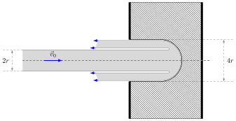
Figure 1: Cross-section of cumulative shell heading towards the armoured wall.

Solution

The problem consists of two parts. The first one asks to explain the phenomenon and the second one asks to determine the speed of the collapsing conical wall that is separating the fuse and the explosive charge of the shell, this collapsing wall is forming the metal jet piercing through the armor. I'll proceed in the order I solved it initially, starting with the part 2.

Part 2

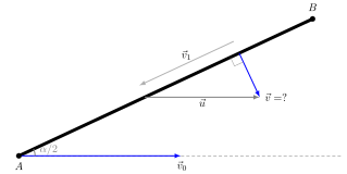
Let's determine the speed of the conical wall collapsing into the jet flowing onto the armor at a speed of $v_{0} = {\rm 8\;km/s}$ as shown in Fig. 2. We focus here only on the upper part of the conical wall cross-section ($AB$, see Fig. 1 as well).

The breaking moment for me here was to realize that the velocity of the conical wall is orthogonal to its surface ($\vec{v}$ in Fig. 2). Since it is collapsing under the pressure force of the gas/liquid created to the left of the cone surface after the explosion of the charge.

Figure 2: Cross-section of the upper part of the collapsing conical wall.

Let's consider a reference frame in which the cone material flows along the cone surface at speed $\vec{v}_1$. This reference frame is moving to the right at a horizontal speed $\vec{u}$, so that the following relation is satisfied:

\begin{equation} \vec{v} - \vec{u} = \vec{v}_1 \end{equation}

In this reference frame the horizontal part of the jet is moving at speed $\left|\vec{v}_1\right| = v_1$ (here and below we ommit the arrow to denote scalar variables). This is relatively easy to prove using energy conservation. In summary we have the following system of equations:

\begin{align} \begin{cases} \vec{v} - \vec{u} = \vec{v}_1\\ v_0 - u = v_1\\ \end{cases} \end{align}

From the triangle formed by the speed vectors in Fig. 2 we get: \begin{align} \begin{cases} v_1 = v / \tan\left(\frac{\alpha}{2}\right)\\ u = v / \sin\left(\frac{\alpha}{2}\right) \end{cases} \end{align}

Now using the last two equations and the relation $v_0 - u = v_1$ we get an equation with respect to $v$:

\begin{align*} v_0 - u = v_1 & \Rightarrow v_0 - v / \sin\left(\frac{\alpha}{2}\right) = v / \tan\left(\frac{\alpha}{2}\right) \\ &\\ & \Rightarrow \boxed{v = \frac{v_0 \sin\left(\alpha/2\right)}{1 + \cos\left(\alpha/2\right)}}\\ &\\ & \Rightarrow v\approx 1.05\:{\rm km/s} \end{align*}

Part 1

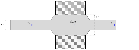
The first part of the problem is to explain the phenomenon, mainly why the speed decreases by a factor of two in the armor. It is more or less clear that the jet will slow down due to the friction with the armor and then will accelerate back behind the armoured wall to the initial speed as it is being pushed forward. The factor of two for the velocity can be explained by the size of the hole pierced by the jet in the armoured wall (as shown in Fig. 3) which is two times larger than the diameter of the jet.

Figure 3: Metallic jet formed from the collapsed conic wall after piercing through the armoured wall, after the stationary flow regime is established.

So now we need to explain why the hole would be approximately twice the size of the metal jet piercing through the armor. For this we need to consider the moments before the hole is pierced completely. At this point there is a part of the jet that flows backwards reflected from the armor as shown in Fig.4 below, which expands the hole. The symmetry and mass conservation would hint us towards the factor of two for the hole diameter.

There is however a question, why would the backflow velocity be directed exactly in the opposite direction with respect to the incident jet. Indeed, this is not obvious.

Figure 4: Metallic jet formed from the collapsed conic wall prior to piercing through the armoured wall.

To find the angle at which the backward flow is reflected we can consider two colliding jets of liquid: smaller with a radius $r$ and a larger one with a radius $R$, moving towards each other at equal and parallel speeds (we can always switch to the reference frame where the metallic jet and the armoured wall move at equal speeds towards each other). As a result of the collision of the jets, a conical backflow in the direction of the smaller jet is formed. If we denote the angle of the cone as $2\beta$, then using momentum, mass and energy conseration it is relatively easy to show that the angle of the cone can be computed using dimensions of the colliding jets as follows: \begin{equation} \cos\beta = \frac{R^2-r^2}{R^2 + r^2} \end{equation}

Now, for our problem if we take the radius of the metallic jet to be $r$, it is much smaller than the effective radius of the armoured wall:

\begin{align} r \ll R & \Rightarrow \cos\beta = \frac{R^2-r^2}{R^2 + r^2} \approx 1 \\ & \Rightarrow \beta \approx 0 \end{align}

which means that indeed in our case the backflow is directed antiparallel to the incident jet velocity.

Physics problem: Horizontal cylindric water pump

First, let me give you the problem statement so you can decide for yourself if the post is worth your time.

Problem statement

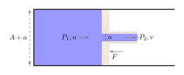
A pump consists of a cylinder with a piston. The cylinder is positioned horizontally. The piston's active pushing area is $A$. There is a hole of area $a$, in the middle of the piston. The piston is pushing water to the left and the water is flowing out to the right through the hole. The force $F$ is applied to the piston to make it move to the left with a constant velocity. Assuming that the flow is laminar and stationary ($\frac{\partial X}{\partial t} = 0$), determine the flow velocity of the liquid through the hole.

[Source: Savchenko et al 1981 physics problems book]

Latex source for the above plot is here: link. In this one I used layers to draw the pump on top of water.

Solution

One thing that we need to realize is that we are asked to compute the outflow speed of the water relative to the piston.

Another one, which is important to get the same answer as in the source physics problem book, is to realize that the total cross-section area of the cylinder is $A+a$.

Now that these two points are clarified we can switch to the reference system moving to the left with the piston. In this reference system the water flows to the right and through the hole. Let's denote the speed of water to the left from the piston and to the right from the piston as $u$ and $v$ respectively. Therefore the speed $v$ is the actual outflow speed we are asked to compute here. Let's denote the pressure to the left and to the right from the piston as $P_1$ and $P_2$ respectively.

Let's write down the following three constraints imposed onto the pump system in the form of equations.

1. The second Newton's law applied to the piston yields:

   $$ F = \left( P_1 - P_2 \right) \cdot A $$

2. The energy conservation law applied to a unit volume of the water (or else known as Bernoulli's law) yields:

   $$ P_1 + \rho \frac{u^2}{2} = P_2 + \rho \frac{v^2}{2} $$

3. The continuity equation yields:

   $$ u \cdot A = v \cdot a $$

Above, we have three equations and three unknowns to be found are $u$, $v$, and $P_1 - P_2$. By solving the above system of equations we obtain the following expression for the outflow speed $v$:

$$ \boxed{v = \sqrt{\frac{2FA}{\rho (A^2 - a^2)}}} $$

Physics problem: Air-filled balloon floating in a rotating cylindrical tank partially filled with water

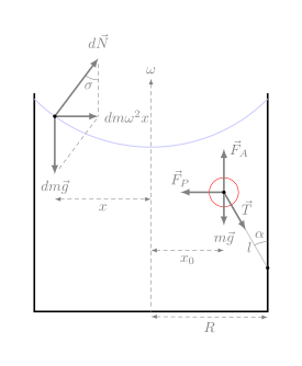
I want to discuss this moderate complexity question about a balloon, filled with air, floating in a rotating tank, which is partially filled with water, as shown in the plot. This is a nice closure for 2023 as it happens to be the last problem on Archimedes' force in the edition of the Savchenko et al problem book that I have. I like this one as its key hint to the solution is in the illustration to the problem.

Problem statement In a cylindrical container, partially filled with water, an air-filled balloon is floating attached to the side wall with a rope as shown in the figure. The container is rotating and the rope is deviated from the side wall towards the center by an angle $\alpha$. The length of the rope is $l$ and the radius of the container is $R$. The radius of the balloon is $r$. Given the information above, determine the angular speed $\omega$ of rotation of the cylinder.

Latex code for the illustration can be found here.

Solution

Before I start describing the solution, I would like to draw your attention to the fact that the balloon is deviated towards the axis of rotation. What would be the reason for this? We need to have a force pulling it towards the center to provide the acceleration towards the rotation axis. It is clear that the rope, attaching the balloon to the wall, pulls the balloon away from the center. Therefore, in principle, I would expect the balloon to be pressed to the side wall of the tank just above the point where the rope is attached to the wall, due to buoyancy of air. And that would probably be true if we had a flat water surface. But here, judging from the illustration, the water surface is not level, but curved, actually its shape is parabolic. This creates a pressure gradient force pushing the air balloon towards the rotation axis.

We can easily compute the pressure gradient at the distance $x$ due to the curvature of the water surface, let's denote the horizontal profile of the water surface as $h(x)$, where $x$ is the distance from the rotation axis on the water surface.

Then

\begin{equation} \frac{\partial P(x)}{\partial x} = \rho_0 g \frac{\partial h(x)}{\partial x} \end{equation}

where $\rho_0$ is the water density, and $g$ is the acceleration due to gravity.

Now, to determine $\frac{\partial h(x)}{\partial x}$ we consider a water parcel at the surface at the distance $x$ from the rotation axis. There are two forces acting on it resulting in the acceleration directed towards the center of rotation: the first one is the reaction of the rest of the water, perpendicular to the water surface as there is no tangent acceleration, and the second one is the force of gravity. It is easy to show that the $\tan$ of the angle between the force of gravity ($dm \vec{g}$) and the reaction force $d\vec{N}$ is:

\begin{equation} \tan\sigma(x) = \frac{\partial h(x)}{\partial x} = \frac{\omega ^ 2 x}{g} \end{equation}

We can use the above to calculate the horizontal pressure gradient as a function of $x$ as follows

\begin{align*} \frac{\partial P(x)}{\partial x} = \rho_0 \cdot \omega ^ 2 x \Rightarrow \\ P(x) = P_0 + \frac{\rho_0 \cdot \omega ^ 2 x ^ 2}{2} \end{align*} where $P_0$ is the pressure at the center of the tank.

So now we would have to find the resulting force, actually the horizontal component of the force, acting on the balloon due to the above pressure field in the water as:

\begin{align*} F_P = \int\limits_{B} P(\beta, \gamma) \cdot \cos \phi(\beta, \gamma) dA \end{align*}

Where $B$ denotes the surface of the balloon, $dA$ is an element of its surface area, $(\beta, \gamma)$ are the angles defining a position of an element $dA$ on the surface of the balloon, and $\phi$ is the angle between the horizontal axis and the normal to the surface of the balloon pointing outside of the balloon (just to have the force positive when it is pushing the balloon towards the center).

It is easy to see that:

$$ dA = r^2\cos\gamma d\gamma d\beta $$

Let's denote the position of the center of the air ballon as $x_0$. We can split the balloon into two equal parts: one closer to the rotation axis and the other one further away from the rotation axis, let's denote water pressure on these parts as $P_{-}(\beta, \gamma)$ and $P_{+}(\beta, \gamma)$.

To fully and independently cover these parts the angles should be $\gamma \in [-\pi/2, \pi/2]$ and $\beta \in [-\pi/2, \pi/2]$. Then we can use $\beta, \gamma$ pair to parameterize the pressure on those sides of the balloon as follows.

$$ P_{+}(\beta, \gamma) = P_0 + \frac{\rho_0 \omega ^ 2}{2}\cdot(x_0 + r \cos\gamma \cdot \cos\beta)^2 $$

And for the half closer to the rotation axis:

$$ P_{-}(\beta, \gamma) = P_0 + \frac{\rho_0 \omega ^ 2}{2}\cdot(x_0 - r \cos\gamma \cdot \cos\beta)^2 $$

Now we pair opposite points with the same $\beta, \gamma$ on both hemispheres to get the contribution to the pressure gradient across the balloon:

$$ \Delta P(\beta, \gamma) = P_{+} - P_{-} = 2 \rho_0\omega^2 r x_0 \cos\gamma \cdot \cos\beta $$

Then the resulting horizontal component of the force acting on the balloon from the two parts is calculated as follows:

\begin{align*} dF_{P} &= \Delta P(\beta, \gamma) dA \cdot \cos\gamma \cos\beta \\ &= 2\rho_0 \omega^2 r^3 x_0 \cos^3\gamma \cos^2\beta d\gamma d\beta \end{align*}

To get the net force we integrate the above expression:

\begin{align*} F_{P} & = 2\rho_0 \omega^2 r^3 x_0 \int\limits_{-\pi/2}^{\pi/2} \cos^3\gamma d\gamma \int\limits_{-\pi/2}^{\pi/2} \cos^2\beta d\beta \\ & = \frac{4}{3} \pi r ^3 \rho_0 \omega^2 x_0 \end{align*}

Now we are ready to write down the second Newton's law projected on the vertical and horizontal axes:

\begin{cases} F_{A} - mg - T \cos\alpha = 0 \\ F_{P} - T \sin\alpha = m \omega ^ 2 x_0 \end{cases}

where $F_{A}$ - is the Archimedes' force acting on the balloon, $mg$ - is the force of gravity pulling the balloon down, and $T$ - is the tension of the rope attaching the balloon to the side wall of the tank.

Let's denote the volume of the balloon as $V$ and the air density as $\rho$, then using the Newton's law expression projected on the vertical axis we can express the tension force as follows:

$$ T = Vg (\rho_0 - \rho) \frac{1}{\cos\alpha} $$

Then we plug the above expression for $T$ in to the equation for the horizontal force components and obtain the following eqaution with respect to the rotation frequency $\omega$:

\begin{align*} T\sin\alpha & = Vg (\rho_0 - \rho) \tan\alpha \\ & = F_{P} - m \omega ^ 2 x_0 = (\rho_0 - \rho) \omega ^ 2 x_0 V \end{align*}

Simplifying the above we get: \begin{align*} g\tan\alpha = \omega ^ 2 x_0 \Rightarrow \omega = \sqrt{\frac{g\tan\alpha}{x_0}} \end{align*}

Now we need to express the distance from the rotation axis to the center of the balloon ($x_0$) through the quantities given in the problem statement. From the geometry considerations it is easy to obtain the following: $$ x_0 = R - (l + r) \sin\alpha $$

Therefore, the final answer to the problem question is:

$$ \boxed{\omega = \sqrt{\frac{g\tan\alpha}{R - (l + r) \sin\alpha}}}. $$

Physics problem: calculating the tension of ropes tying together timbers of a raft

This problem comes from my usual source of inspiration, the book by Savchenko et al., from the section on floating bodies and Archimedes' force. I spent a considerable amount of time figuring this one out, mostly because the answers in the edition I have and in the newer edition do not match. Another reason I could not get the correct answer is that I did not think that we should account that there are actually two ropes one at the front and the second is at the back of the raft.

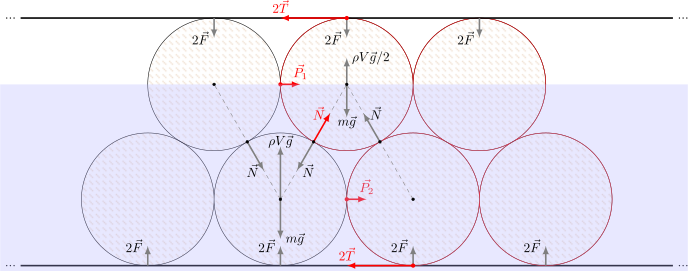
Here is the problem statement: Consider two rows of wooden timbers tied together into a raft, as shown in the figure. Half of the top row of the timbers is above the water surface. Determine the minimum tension of the two ropes holding the timbers together, if the mass of each timber is $m$. The raft is very wide.

Solution

Let's denote water density as $\rho$ and the volume of each timber as $V$. Let's refer to forces, acting between the timbers and between a tibmer and a rope as $N$ and $F$ respectively. See the figure below (the Latex code for the fiigure can be found here).

We can express the equillibrium of a bottom and of a top timbers separately using vertical components of forces acting on them:

$$\tag{1} \begin{cases} 2F - N\sqrt{3} - mg + \rho V g = 0 \\ -2F + N\sqrt{3} - mg + \frac{1}{2} \rho V g = 0 \end{cases}\\ \Rightarrow -6F + 3N\sqrt{3} - mg = 0 $$

Note that we have $2F$ in each of the equations above for the force the ropes push timber downwards or upwards because we have two ropes one at the front and another at the back of the raft.

Let's consider vertical components of the forces acting on the upper part of one of the ropes. Assuming that we have around $n$ timbers in each row and that the mass of the rope is negligible, we get:

\begin{equation}\tag{2} n \cdot F = 2 T\cos\alpha \end{equation}

Where $\alpha$ - is the angle of the tension force with the vertical at the left and right edges of the raft. The tension arises from the bottom part of the rope pulling the upper part down. Since the $n$ is large, according to the problem statement, we can deduce:

\begin{equation}\tag{3} F = 2 \frac{T\cos\alpha}{n} \rightarrow 0 \end{equation}

So the equation (1) simplifies to the following: \begin{equation}\tag{4} 3 N\sqrt{3} - mg = 0 \end{equation}

Now let's consider the right part of the timbers as a system and write down the equillibrium condition for horizontal components of the forces acting on it. I highlighted in red the timbers in the selected system as well as relevant forces:

\begin{equation}\tag{5} \frac{N}{2} + P_1 + P_2 - 4T = 0\\ \Rightarrow 4T = \frac{N}{2} + P_1 + P_2 \end{equation}

where $P_1 \geq 0$, and $P_2 \geq 0$ - horizontal forces exerted by the neighbour timbers from the top and the bottom rows respectively onto the above selected system of the timbers.

Therefore,

\begin{equation}\tag{6} 4 T \geq \frac{N}{2} \Rightarrow T_{\min} = \frac{N}{8} \Rightarrow N = 8 T_{\min} \end{equation}

Then substituting the above expression for $N$ into equation (4) we get:

\begin{equation}\tag{7} 24 T_{\min}\sqrt{3} - mg = 0 \\ \Rightarrow \boxed{T_{\min} = \frac{mg}{24\sqrt{3}} = \frac{mg\sqrt{3}}{72}} \end{equation}

The above result is the same as in the newer edition of the book. At this point, I am not sure how the answer in the old edition of the book was obtained, because if we forget about one rope, the $T_{\min}'$ would be two times greater then the correct one, but in the older edition the tension is $4 T_{\min}$ for some reason....

Stability of a rectangular box floating on a surface of a liquid

This problem, as many of the previous discussed here, is coming from the Savchenko et al book. It took me around one month to wrap my head around this one. I have to admit that I improved (or refreshed) my knowledge of Archimedes' force thanks to this one. Specifically, this problem highlights the fact that Archimedes' force is applied to the center of mass of the water replaced by a floating object. Therefore, even if the object's density is uniform, it can happen that the torques of the gravity force and the Archimedes' force are not compensated even though the modules of the forces are equal. This fact makes more interesting the question about stability of a floating object in a liquid.

Problem statement

Given a rectangular body of length $a$, width $a$, and height $b$. Its density is $\rho$ and it floats in a liquid of density $\rho_0$. Determine the ratio $\frac{a}{b}$ for which the object's equillibrium state is stable. It is assumed that the side $b$ of the box is vertical in the equillibrium position.

Discussion

It is obvious that the object's equllibrium is stable with respect to vertical displacements, because if we push it down, the Archimedes' force increases and pushes it back. Similarly, if we pull the object up, the Archimedes' force becomes smaller and the gravity pushes it back to its initial equillibrium position where the gravity force is compensated by the Archimedes' force. Therefore, further down we consider only stability of the object with respect to rotations.

We won't consider the case with the box completely submerged into the liquid as in this case the center of mass of the box coincides with the center of mass of the liquid pushed out by the box, due to the uniform density of the box, and therefore the net torque (exerted by the gravity and Archimedes' forces) will always be zero. I guess this case is not stable with respect to rotations, as the box won't be restored to its original vertical position. Zero gravity, like in the outer space, all orientations are equivalent.

Here we can speculate a bit. Intuitively we would expect that the larger base (i.e. greater $a$) with respect to the height $b$ would give us a more stable equillibrium. Hence we can expect the result to be in a form $\frac{a}{b} > r$ or $\frac{a}{b} \geq r$.

Let's denote the height of submerged part of the box as $h$ and the pivot point as $O$. The pivot point is the intersection of the vertical axis of symmetry of the box and the horizontal plane at the level of the surface of the liquid (the updated level after the box is submerged), see the figure below. We consider rotations at a small angle $\varphi$ around this pivot point $O$.

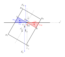
The latex source for the plot can be found here.

There are two ways to find out if the vertical upright orientation of the box is stable: using the change in the height of the center of mass of the system liquid and box, i.e., if the above rotations lower the center of mass of the system then its vertical orientation is not stable, otherwise it is stbale, and using the net torque exerted by the gravity and Archimedes' forces, i.e., in the stable case the torque would act in the direction opposite to the direction of rotation,otherwise it is not stable. We'll use both methods and compare the results.

But first let's prepare a few useful expressions. If we denote as $A$ the center of mass of the liquid pushed out by the box (this is also the point where the Archimedes' force is applied to the box). Let's determine its coordinates $\left(x_{A\varphi}, y_{A\varphi}\right)$ when the box is rotated, in the system of coordinates with the center at the point $O$ and the $y$-axis pointing downward and the $x$-axis pointing to the right. It is easy to see that the mass ($m_A=\rho_0 a^2 h$) of the liquid pushed out by the box does not change during the rotation as well as the module of the Archimede's force $F_A=m_A g$. By definition, expressions for the coordinates of the center of mass of the liquid pushed out by the box can be written as:

\begin{cases} m_A x_{A\varphi} = m_A x_{A'\varphi} + m_L x_L + m_R x_R \\ m_A y_{A\varphi} = m_A y_{A'\varphi} + m_L y_L + m_R y_R \end{cases}

where

\begin{align} m_L = -m_R\\ x_L = -x_R\\ y_L = -y_R\\ \end{align}

and the $A'\varphi$ is the center of mass of the fictious liquid volume when it is rotated from the upright position as a solid body, $m_L$ and $m_R$ are the masses of the prisms (triangles in 2D, see the above figure) to be removed from and added to the fictious liquid body respectively to get the real shape of the liquid pushed out by the box during rotation. $\left(x_R, y_R\right)$ and $\left(x_L, y_L\right)$ are the centers of mass of the prisms of masses $m_R$ and $m_L$ respectively (red and blue triangles in the figure, the blue one has negative mass and the red one has positive mass). Since $m_L$ is the mass to be removed, it is negative in the equations to avoid confusion with the signs. We use these triangles (prismes in 3D) to facilitate the calculation of the position of the center of mass of the liquid pushed out by the box $A\varphi$. It is easy to compute coordinates of the center of mass of the fictious rectangular volume $B_1B_2RL$ and then to find coordinates of $A\varphi$ (of the complex shape of the liquid pushed out by the rotated box) we compute the center of mass of a system consisting of $B_1B_2RL$, $m_R$ and the negative mass $m_L$. The center of mass of such a system is $A\varphi$. If we substitude the relations between $m_L$ and $m_R$ into the equations for $x_{A\varphi}$, $y_{A\varphi}$ we get the following expressions:

\begin{cases} x_{A\varphi} = x_{A'\varphi} + 2 \frac{m_R}{m_A} x_R \\ y_{A\varphi} = y_{A'\varphi} + 2 \frac{m_R}{m_A} y_R \end{cases}

It is easy to see that

\begin{align} \frac{m_R}{m_A} & = \frac{\rho_0 \frac{1}{2}\cdot \frac{1}{2} a \cdot \frac{1}{2} a \tan\varphi\cdot a}{\rho_0 a^2 h} = \ \frac{a}{8h}\tan\varphi \approx \frac{a}{8h}\varphi \\ x_{A'\varphi} & = -\frac{h}{2}\sin\phi \approx -\frac{h}{2}\phi\\ y_{A'\varphi} & = \frac{h}{2}\cos\phi \end{align}

We keep exact values for the $y$ coordinates here as the changes in $y$ due to the rotation are on the order of $\sim\varphi^2$ and the variations of $x$ coordinates are on the order of $\sim\varphi$.

From the geometry and the properties of the centre of mass of a triangle we can determine $x_R$ and $y_R$: \begin{cases} x_R & = \frac{a}{2\cos\varphi}\cdot\frac{1}{2} + \frac{1}{3} \frac{a}{2\cos\varphi} \cos2\varphi = \frac{a}{4\cos\varphi}\left(1 + \frac{\cos2\varphi}{3}\right)\\ y_R & = \frac{1}{3}\left(\frac{a}{2\cdot2\cos\varphi}\right)\sin2\varphi = \frac{1}{6}a\sin\varphi \end{cases}

For small angles $\varphi$ (which is the case in the problem at hand), we get the following expressions for $x_R$ and $y_R$:

\begin{cases} x_R & \approx \frac{a}{3} \\ y_R & \approx \frac{a}{6}\varphi \end{cases}

Using the above relation we can express $\left(x_{A\varphi}, y_{A\varphi}\right)$ as functions of $h$, $a$, and $\varphi$:

\begin{cases} x_{A\varphi} = x_{A'\varphi} + 2 \frac{m_R}{m_A} x_R \approx -\frac{h}{2}\phi + 2 \frac{a}{8h}\varphi \cdot \frac{a}{3} = \frac{\varphi}{4h}\left( \frac{a^2}{3} - 2 h^2 \right)\\ y_{A\varphi} = y_{A'\varphi} + 2 \frac{m_R}{m_A} y_R \approx \frac{h}{2}\cos\varphi + 2 \frac{a}{8h}\varphi \cdot \frac{a}{6}\varphi = \ \frac{h}{2}\cos\varphi + \frac{a^2}{24h}\varphi^2 \end{cases}

We did not replace $\cos\varphi$ with one for the $y$ coordinate since the accuracy of the terms is $\varphi ^ 2$.

Let's note the coordinates of the center of mass of the pushed out liquid for $\varphi=0$:

\begin{cases} x_{A0} = 0\\ y_{A0} = \frac{h}{2} \end{cases}

It is easy to derive how the coordinates of the center of mass of the box ($C$) change during rotation, as it is always in the middle of the box:

\begin{cases} x_{C\varphi} = \left( \frac{b}{2} - h \right)\sin\varphi\\ y_{C\varphi} = \left( h - \frac{b}{2} \right)\cos\varphi \end{cases}

Finally, let's express $h$ using equillibrium between the Archimedes' ($F_A$) and the gravity ($F_C = m_C g$) forces:

\begin{align} F_C-F_A=0 \Rightarrow \rho a^2 b - \rho_0 a^2 h = 0 \Rightarrow h=\frac{\rho}{\rho_0}b \end{align}

Method 1: analysis of torques

Without the loss of generality we can consider clockwise rotation as shown in the plot. Torques acting in the counter-clockwise direction are positive and torques acting in the clockwise direction are negative. With this convention, for stability it is required that the net torque ($\tau$) should act in the direction opposite to the rotation (i.e. anti-clockwise). Therefore the condition for stability is $\tau > 0$.

Let's consider two cases and impose the stability condition:

a) the center of mass is below the liquid surface $h\geq b/2$

If $x_{A\varphi} \geq 0$, then $\tau = F_C |x_{C\varphi}| + F_A |x_{A\varphi}|$, which is always positive. Both $\tau_C$ and $\tau_A$ act to stabilize the box against rotation.

If $x_{A\varphi} < 0$, then stability condition is:

\begin{align} \tau = F_C |x_{C\varphi}| - F_A |x_{A\varphi}| > 0 \end{align}

Since $F_C = F_A$ (as well as $m_A = m_C$), for stability we need the following:

\begin{align} |x_{C\varphi}| - |x_{A\varphi}| > 0 &\Rightarrow - \left( \frac{b}{2} - h \right)\varphi - (-1)\cdot\frac{\varphi}{4h}\left( \frac{a^2}{3} - 2 h^2 \right) > 0 \\ & \Rightarrow -\frac{b}{2} + h + \frac{1}{4h}\left( \frac{a^2}{3} - 2 h^2 \right) > 0 \\ & \Rightarrow -2bh + 4h^2 + \frac{a^2}{3} - 2 h^2 > 0 \\ & \Rightarrow -6bh + a^2 + 6 h^2 > 0 \\ & \Rightarrow -6b^2\frac{\rho}{\rho_0} + a^2 + 6 \left(\frac{\rho}{\rho_0} b\right)^2 > 0 \\ & \Rightarrow \left(\frac{a}{b}\right)^2 > 6\frac{\rho}{\rho_0} - 6 \left(\frac{\rho}{\rho_0} \right)^2 \\ & \Rightarrow \boxed{\frac{a}{b} >\sqrt{ 6\frac{\rho}{\rho_0}\left(1 - \frac{\rho}{\rho_0} \right) }} \end{align}

b) the center of mass is above the liquid surface $h < b/2$

In this case the gravity force acts to destabilize the box with its torque acting in the direction of rotation. So the stability in this case is possible when $|x_{A\varphi}| > |x_{C\varphi}|$ and $x_{A\varphi} \cdot x_{C\varphi} > 0$ (i.e. A and C are from the same side from the pivot point $O$) which is equivalent to:

\begin{align} \tau = -F_C |x_{C\varphi}| + F_A |x_{A\varphi}| > 0 &\Rightarrow \ - (-1) \cdot \left(h - \frac{b}{2}\right)\varphi + \frac{\varphi}{4h}\left( \frac{a^2}{3} - 2 h^2 \right) > 0 \\ &\Rightarrow \boxed{\frac{a}{b} >\sqrt{ 6\frac{\rho}{\rho_0}\left(1 - \frac{\rho}{\rho_0} \right) }} \end{align}

Let's check if the conditions we imposed do actually make sense.

\begin{align} h < b/2 \Rightarrow \rho/\rho_0 < 1/2 \Rightarrow a/b > \sqrt{3/2} \Rightarrow \frac{a^2}{3} - \frac{b^2}{2} > 0 \Rightarrow x_{A\varphi} > 0 \end{align}

remembering that we consider only $\varphi > 0$.

Method 2: minimum of the potential energy of the system

I like this method more as it requires less logic branching. Let's denote as $y$ the $y$-coordinate of the center of mass of the system liquid and box. Since the positive direction of the axis is downwards, the change $\Delta y < 0$ during the rotation of the box would mean that the center of mass of the system is lifted and therefore the system's potential energy would be increasing and the system itself will tend to minimize its potential energy, therefore $\Delta y < 0$ is our stability condition. By the definition of the center of mass we have:

\begin{align} (M - m_A + m_C) y = m_C y_{C\varphi} - m_A y_{A\varphi} + M y_0 \end{align}

where $M$ is the mass the liquid would have when the immersed part of the box is replaced by the liquid. $y_0$ is the $y$-coordinate of the center of mass of $M$.

Let's examine the change in the $y$-coordinate of the center of mass of the system during rotation:

\begin{align} \Delta y = \frac{1}{M - m_A + m_C}\left ( m_C \Delta y_{C} - m_A \Delta y_{A} \right) \Rightarrow \Delta y \propto m_C \Delta y_{C} - m_A \Delta y_{A} \end{align}

Noting that $m_C = m_A$, we get:

\begin{align} \Delta y \propto \Delta y_{C} - \Delta y_{A} \end{align}

Therefore the condition for the system stability is equivalent to:

\begin{align*} \Delta y < 0 \Rightarrow \Delta y_{C} - \Delta y_{A} < 0 \end{align*}

From the relations prepared above we can express $\Delta y_{C}$ and $\Delta y_{A}$ as follows:

\begin{align*} \Delta y_{A} & = y_{A\varphi} - y_{A0} = \frac{h}{2}\cos\varphi + \frac{a^2}{24h}\varphi^2 - \frac{h}{2} = \frac{a^2}{24h}\varphi^2 - \frac{h}{4} \varphi^2 \\ \Delta y_{C} & = y_{C\varphi} - y_{C0} = \left(h - \frac{b}{2}\right)\left(\cos\varphi - 1 \right) \approx -\left(h - \frac{b}{2}\right)\frac{2\varphi^2}{4} \end{align*}

Now plugging the above expressions for $\Delta y_{C}$ and $\Delta y_{A}$ into the stability inequality, we get:

\begin{align*} & -\left(h - \frac{b}{2}\right)\frac{2\varphi^2}{4} - \frac{a^2}{24h}\varphi^2 + \frac{h}{4} \varphi^2 < 0 \Rightarrow \\ & \Rightarrow \frac{b}{4}\varphi^2 - \frac{h}{4} \varphi^2 - \frac{a^2}{24h}\varphi^2 < 0 \Rightarrow \\ & \Rightarrow 6 (b - h) h - a^2 < 0 \Rightarrow 6 \frac{\rho}{\rho_0} \left( 1 - \frac{\rho}{\rho_0} \right) b^2 - a^2 < 0 \Rightarrow \\ & \Rightarrow \boxed{\frac{a}{b} > \sqrt{6 \frac{\rho}{\rho_0} \left( 1 - \frac{\rho}{\rho_0} \right)}} \end{align*}

In conclusion, we are happy that the minimum potential energy and the torque methods give the same result.

\begin{equation*} \boxed{\frac{a}{b} > \sqrt{6 \frac{\rho}{\rho_0} \left( 1 - \frac{\rho}{\rho_0} \right)}} \end{equation*}

Sound waves in an ocean column

This problem is about infrasound oscillations in an ocean column, it is taken from Savchenko et. al. (1981). And the question is as follows.

What ocean depth would allow development of physiologically dangerous infrasound oscillations at a linear frequency of $\nu=7\;{\rm Hz}$.

My approach is to examine modes allowed by the ocean column assuming that we have a displacement node at the ocean floor and a displacement antinode at the ocean surface. That is when a forced oscillation is excited by some external forcing (e.g wind) only the modes corresponding to the natural (eigen) frequencies would be reinforced by a resonance. I assume that we have an antinode at the surface as the surface is much less constrained than the deeper water layers.

Using a general equation for the modes (also known as standing waves, which could be combined to approximate any solution to the wave equation, provided the standing wave components satisfy imposed boundary conditions). The displacement $\Psi_m(z, t)$ in such a standing wave is expressed as follows, assuming $z=0$ at the bottom of the ocean.

\begin{equation} \Psi_m(z, t) = A_m \sin \left( k_m z \right) \sin\left(\omega_m t + \alpha_m \right) \end{equation}

Where $k_m=\frac{\omega_m}{c}=\frac{2\pi\nu_m}{c}$ and $c$ - is the speed of sound in the ocean. It is interesting to note here that all the points in the standing wave oscillate at the same frequency $\omega_m$.

These $\Psi_m(z, t)$ automatically satisfy the node condition at the ocean floor. Now we are interested in the frequencies $\nu_m=\nu=7\; {\rm Hz}$ and impose the antinode condition at the ocean surface, i.e. $z=H_n$:

\begin{equation} \sin \left( k_m H_n \right) = 1 \Rightarrow k_m H_n = \frac{\pi}{2} + n \pi \end{equation}

where $n = 0,1,2,3,... $.

From the above we can determine $H_n$, by setting $\nu_m = \nu$:

\begin{split} k_m H_n = \frac{\pi}{2} + n \pi & \Rightarrow \\ \frac{2\pi\nu_m}{c} H_n = \frac{\pi}{2} + n \pi & \Rightarrow \\ H_n=\frac{c}{4 \nu} \left(2 n + 1 \right) \end{split}

The above results approximately (assuming $c\approx 1500 \; {\rm m/s}$) in the following values for the ocean depth

\begin{split} & H_0 = 50\;{\rm m} \\ & H_1 = 150\;{\rm m} \\ & H_2 = 250\;{\rm m} \\ & H_3 = 350\;{\rm m} \\ & H_4 = 450\;{\rm m} \\ & ... \end{split}

Which looks ok to me, but unfortunately this is not the answer given in the book, and it really annoyed me for some time. And I am still not sure why but the authors advance that $H_n = \frac{c}{4 \nu} \left(4 n + 1 \right)$ instead of the $H_n = \frac{c}{4 \nu} \left(2 n + 1 \right)$ obtained above. It seems like the depths $H_n = \frac{c}{4 \nu} \left(4 n - 1 \right)$ are not suitable for some reason. If someone can explain this to me, that would be great ... But for now I am leaving it here hoping that maybe they simply forgot to consider these solutions.

Phase speed of gravity waves in a shallow water layer

This is something I probably heard many times at many courses I was attending during my long years of studies. Nevertheless, I don't think I really understood what was going on physically, although I have never had problems understanding mathematics involved, i.e. equations were clear as well as transformations required to linearize them, for example to get a wave dispersion relation $\omega=\omega(k)$.

Currently, I am going (slowly) through the deformations section ("Deformations and Strains. Wave speed") in my favourite physics problem book (Savchenko et al 1981) and one problem is asking to derive an expression for the phase speed of gravity waves in a shallow water layer, assuming the wave lengths to be much larger than the depth of the water layer. Another implied condition is that the density of the fluid is constant so that we indeed focus only on gravity waves, because a fluid with varying density would allow for elastic waves (I hope this is the right term here...).

I was trying to think of perturbations and how they would be propagating and about trajectories of water parcels subjected to the above constraints (mostly mass conservation). But honestly I could not understand right away how to go about solving the problem without formally writing equations of motion and actually got some help and direction from "Essentials of Atmospheric and Oceanic Dynamics" by Geoffrey Vallis. When I finally clearly realized the path for this formal solution I wrote it down as follows.

Figure 1 shows the water layer and a perturbation propagating to the right at speed $c$.

Considering the problem to be one-dimensional with the $x$-axis pointing towards the direction of the propagation of waves, we can write the following linearized momentum and mass continuity equations.

$$ \left\{\begin{array}{l} \partial_t u &= -\frac{1}{\rho_0}\partial_x P = -g \partial_x \eta \\ \partial_t \eta &= -h \partial_x u \end{array}\right.\tag{1} $$

These $u$ ($x$-component of the current) and $\eta$ (elevation relative to the unperturbed depth $h$) are small perturbations around the base state of the shallow water layer at rest. The impact of Earth rotation is ignored here, you could checkout "Essentials of Atmospheric and Oceanic Dynamics" for more details about the Earth rotation effects (i.e. Coriolis force).

Then by applying $\partial_x$ and $\partial_t$ to the first and the second equations of the system (1) respectively we obtain the following equation for $\eta$:

$$ -\frac{1}{h} \partial_{t}^2 \eta = -g\partial_{x}^2\eta \Rightarrow \\ \boxed{\frac{1}{gh} \partial_{t}^2 \eta = \partial_{x}^2\eta} $$

Comparing the above to the canonical wave equation

$$ \frac{1}{c^2}\partial_t^2 \xi = \partial_{x}^2\xi + \partial_{y}^2\xi + \partial_{z}^2\xi = \Delta \xi $$

we can conclude that the wave speed in our case is $c=\sqrt{gh}$. Note how it does not depend on $k=2\pi/\lambda$, i.e. the same for all wavelengths, so that the initial perturbation won't be deforming and would maintain its shape with time. This is not the case for waves in deep water.

That would close the problem for me and I would move on, but somehow I decided to dig a bit around and learned a bit more about these waves in Feynman's physics lectures, although he was considering short waves in a very deep layer (even considering capillary effects). There he describes water parcel trajectories which are not that simple as one can think. In Feynman's book and at the back of the problem book itself I found hints to the following simpler solution of this problem.

This alternative approach is visualised in Figure 2.

Assuming that we have a limit between unperturbed and perturbed parts of the fluid propagating with speed $c$ (the one we are interested to compute). Let's denote the height difference between these parts of the fluid as $\Delta h$. If we accept that water from the perturbed region would pile onto the water from the unperturbed region, we could express the water flux as follows:

$$ u(h + \Delta h) = c \Delta h $$

We can simplify this expression using the assumption that $\Delta h \ll h$ and therefore:

$$ uh = c \Delta h \Rightarrow u = c \frac{\Delta h}{h} \tag{2} $$

Now we can use momentum equation to get more information about propagation of the perturbed region. During time $\Delta t$ a part of the unperturbed region will gain the same speed as in the perturbed region and we can write the momentum change as follows:

$$ \Delta p = \rho_0 c \Delta t h \Delta y \cdot u \Rightarrow \frac{\Delta p}{\Delta t} = \rho_0 c h \Delta y \cdot u $$

This momentum change is caused by the pressure of the perturbed region on the unperturbed region:

$$ F = \rho_0 g \Delta h \cdot \Delta y h = \rho_0 c h \Delta y \cdot u $$

Then simplifying we get

$$ g \Delta h = c \cdot u $$

And substituting $u$ from equation (2) we get the following:

$$ g \Delta h = c \cdot c \frac{\Delta h}{h} \Rightarrow c=\sqrt{gh} $$

Physics problem: ocean compressibility

This problem is not complicated, but it is particularly interesting to me as it is related to my work: modelling of the ocean, especially dynamics and everything impacting water level. I took it from the book by Savchenko et al., in the section on deformations.

Problem statement

Assuming that compressibility of water is $\alpha=5\times 10^{-10}\; {\rm Pa^{-1}}$ and the mean ocean depth is around 3.5 km, answer the following questions:

1. Estimate the change in water level if water becomes incompressible.
2. At some places the ocean is 10 km deep. Estimate the change of water density between the 10 km depth and the surface.
3. What is the deformation energy stored in 1 ${\rm m^3}$ of water at the 10 km depth?

Solution

It is probably easy to show that the weight of atmosphere is negligible in comparison with the weight of water pushing and compressing the ocean. Therefore I will neglect the impacts of atmospheric pressure for this problem and will assume that the only cause for the compression of the ocean is its weight.

First, let's remember the definition of the compressibility coefficient, i.e. relative change of volume per unit change of pressure:

\begin{align} \frac{dV}{V} = -\alpha \cdot dP \end{align}

where $V, P$ are the volume and pressure respectively.

To answer the above questions we would need to know how the density of water changes with depth, i.e. $\rho(z)$. We select a layer at depth $z$, and if we push it down by $dz$, the pressure would increase by $dP = \rho(z)\cdot g dz$, since we would have additional amount of water pushing down on our layer. This same pressure increase can be expressed using the definition of compressibility coefficient:

$$ dP = \rho(z)\cdot g dz = \frac{dV}{\alpha V} $$

Then using the relation $V(z) = \frac{m}{\rho(z)}$ and the fact that the mass does not vary during compression, we can express the relative volume change as:

$$ \frac{dV}{V} = \frac{d(m/\rho(z))}{m/\rho(z)} = \frac{d(1/\rho(z))}{1/\rho(z)} \Rightarrow \\ dP = \rho(z)\cdot g dz = -\frac{d(1/\rho(z))}{1/\rho(z) \cdot \alpha} = -\frac{\rho(z)}{\alpha}d\left( \frac{1}{\rho(z)} \right) $$

Then simplifying we get the following equation for the function $\rho(z)$:

$$ d\left( \frac{1}{\rho(z)} \right) = -\alpha g dz $$

Integrating and denoting surface water density as $\rho_0$:

$$ \frac{1}{\rho(z)} = -\alpha g z + \frac{1}{\rho_0} \Rightarrow \\ \rho(z) = \frac{1}{-\alpha g z + \frac{1}{\rho_0}} \Rightarrow \\ \rho(z) = \frac{\rho_0}{1 - \alpha \rho_0 g z} $$

It is easy to estimate that the product in the denominator is at most

$$ \alpha \rho_0 g z \lesssim 10^{-10} \cdot 10^3 \cdot 10^4=10^{-3} \ll 1 $$

Therefore we can further simplify the expression for $\rho(z)$:

\begin{align} \rho(z) \approx \rho_0 \left(1 + \alpha \rho_0 g z \right) \end{align}

Q1: Estimate change in water level if water becomes incompressible.

To figure out the change of the water level we divide the ocean into horizontal layers of width $dz$ and then we calculate compression of each layer due to the weight of water above it. Finally, we can find the water level rise by summing the compressions for all layers.

Following the above plan, we can express mass per unit area of the water layer $dz$ as below:

$$ d\mu = \rho(z)dz = \rho_0 (dz + dh) $$

where $dh$ is the increase of the water layer width due to decreased pressure at the surface (i.e. $P(z=0)=0$).

By reorganizing the terms in the equation above we get:

$$ (\rho(z) - \rho_0) dz = \rho_0 dh $$

Now we substitute the expression we obtained previously for $\rho(z)$ :

$$ \frac{\rho(z) - \rho_0}{\rho_0} dz = dh \Rightarrow \\ \alpha\cdot \rho_0 g z dz = dh $$

Then by integrating from the surface ($z=0$) down to the mean water depth ($z=\overline{H}$), we find the total compression of the water layers, if there was no weight pushing on them, which is equivalent to the problem statement condition imposing water incompressibily:

$$ \Delta h = \int\limits_{0}^{\Delta h} dh = \int\limits_{0}^{\overline{H}}\alpha\cdot \rho_0 g z dz = \alpha\cdot \rho_0 g \frac{\overline{H}^2}{2} \Rightarrow \\ \boxed{ \Delta h \approx 5 \cdot 10^{-10} \cdot 10^3 \cdot 10 \cdot \frac{3.5^2\cdot 10^6}{2} \approx 30.6 \;({\rm m})} $$

Finally, we obtain that if water in the ocean becomes incompressible, the water level will rise by about 30 meters.

Q2: At some places the ocean is 10 km deep. Estimate the difference of water density between the 10 km depth and the surface.

The answer to this question directly follows from the expression we derived for $\rho(z)$ in the beginning of the post:

$$ \Delta\rho (z) = \rho(z) - \rho_0 = \alpha \rho_0^2 g z $$

where $\Delta\rho (z)$ is the difference of water density between the depth $z$ and the surface.

If we substitute 10 km depth (i.e. $z_1 = 10^4 \; {\rm m}$):

$$ \boxed{ \Delta\rho (z_1) = \alpha \rho_0^2 g z = 5 \cdot 10^{-10} \cdot 10^6 \cdot 10 \cdot 10^4 = 50\;({\rm kg/m^3}) } $$

Q3: What is the deformation energy stored in 1 ${\rm m^3}$ of water at the 10 km depth?

The deformation energy stored in comressed water can be computed using work needed to compress a water parcel (let's say a unit cube) from its density at the surface to its density at the 10 km depth. It is easy to show that the compression work $dW$ can be expressed as follows:

$$ dW = PdV \Rightarrow W = \int\limits_{V_0}^{V_H} PdV $$

Using the expression for the compression coefficient we can find pressure as a function of volume $P(V)$:

$$ \int \frac{dV}{V} = -\alpha dP \Rightarrow \ln V = -\alpha P + C $$

Using that at the surface $P(z=0) = 0$ (actually it is equal to the atmospheric pressure, but we neglect it compared to the weight of water) and denoting the volume of the water parcel at the surface as $V_0$ we get:

$$ P = -\frac{1}{\alpha} \ln\frac{V}{V_0} $$

Now we plug it into the expression for work $W$:

\begin{align*} W =& \int\limits_{V_0}^{V_H} -\frac{1}{\alpha} \ln\frac{V}{V_0} dV \\ =& -\frac{V_0}{\alpha} \int\limits_{1}^{V_H/V_0} \ln y \cdot dy \\ =& -\frac{V_0}{\alpha} \left( \left. \ln y \right\rvert_{1}^{V_H/V_0} - \frac{V_H}{V_0} + 1 \right) \\ =& -\frac{V_0}{\alpha} \left( \ln \left( \frac{V_H}{V_0}\right) - \frac{V_H}{V_0} + 1 \right) \\ \end{align*}

Using the relation between densities and volumes of the same parcel of water and expressing the density difference calculated in Q2 we get:

$$ \frac{V_H}{V_0} = \frac{\rho_0}{\rho_H} = \frac{\rho_0}{\rho_0 + \alpha \rho_0^2 g H} = \frac{1}{1 + \alpha \rho_0 g H} $$

Then we can plug the volume ratio into the expression for the energy and get the density as follows:

\begin{align*} \omega & = \frac{W}{V_H} \\ & = -\frac{V_0}{\alpha V_H} \left( \ln \left( \frac{V_H}{V_0}\right) - \frac{V_H}{V_0} + 1 \right) \\ & = -\frac{1 + \alpha \rho_0 g H}{\alpha} \left( -\ln \left( 1 + \alpha \rho_0 g H\right) - \frac{1}{1 + \alpha \rho_0 g H} + 1 \right) \\ \end{align*}

Then using that the $\alpha \rho_0 g H$ is much smaller than 1 as was shown above, we can do the following approximations to the second order of $\alpha \rho_0 g H$:

\begin{align*} \omega & \approx -\frac{1 + \alpha \rho_0 g H}{\alpha} \left( -\alpha \rho_0 g H +\frac{\left(\alpha \rho_0 g H\right)^2}{2} - (1 - \alpha \rho_0 g H + \left(\alpha \rho_0 g H\right)^2) + 1 \right) \\ & = -\frac{1 + \alpha \rho_0 g H}{\alpha} \left( -\frac{\left(\alpha \rho_0 g H\right)^2}{2}\right)\\ & \approx \frac{\alpha}{2}\left( \rho_0 g H\right)^2 \end{align*}

Therefore, the deformation energy density of water at the depth $H$ can be approximated as follows:

$$ \boxed{ \omega = \frac{\alpha}{2}\left( \rho_0 g H\right)^2 } $$

Now, substituting values we get that at the depth $H=10 {\rm km}$:

$$ \omega \approx 0.5 \cdot 5 \cdot 10^{-10}\cdot 10^6 \cdot 10^2 \cdot 10^8=\underline{2.5\times10^6\;({\rm J/m^3})} $$

Minimum work required to bend a metal rod

This problem is from the section on deformations obbeying the linear relation between reaction force and deformation length. This one requires knowledge of Young modulus which allows to express reaction force as a function of relative deformation. In one-dimensional case the law looks as follows:

$$ \sigma = E\varepsilon $$

where $\sigma=F/A$ is the reaction tension (${\rm N/m^2}$) of the material in response to the relative deformation $\varepsilon=\Delta L / L$.

This problem is taken from the book Savchenko et al and it took me some time to understand to my satisfaction, therefore it is written up here.

Problem statement

Determine the minimum amount of work required to bend a rod of length $l$ with square cross section ($a \times a$) into a ring. Young modulus of the material is $E$ and $l \gg a$.

Solution

The approach to take here was hinted to me by the previous problem which asked for the expression of the energy density for a deformed material. It is relatively easy to derive using the above expression for the deformation tension that the energy density per unit volume ($\omega$) can be expressed as follows:

$$ \omega = \frac{dW}{dV} = \frac{E\varepsilon^2}{2} $$

So the problem now is reduced to finding the ring configuration that would minimize the energy (work) due to deformation of the rod:

$$ W = \int\omega dV \Rightarrow W_{\rm min} = \min_{V_{\rm ring}}\left( \int \omega dV \right) $$

In the bent state we can divide the ring into multiple strips of width $dr$ with the smallest having the radius $R$. We assume that the length of the longest (outer) strip would be $R+a$, i.e. here we neglect radial deformations and assume that the width of the rod as well as its height won't change. Then the deformation energy $dW$ stored in each strip would be:

$$ dW = \omega dV = \frac{E\varepsilon^2}{2}dV =\frac{E\varepsilon^2}{2}a\cdot 2\pi r dr $$

Therefore the total energy of the deformed rod would be a sum of energy of each of the strips:

$$ W = \int\limits_{R}^{R+a}\frac{E\varepsilon^2}{2}a\cdot 2\pi r dr $$

Then noting that for each strip the relative deformation $\varepsilon$ is $(2 \pi r -l )/l $, we get: $$ W(R) = \int\limits_{R}^{R+a}\frac{E(2 \pi r - l)^2}{2l^2}a\cdot 2\pi r dr $$

Now we need to find the radius of the shortest strip $R$ (which would also define the radii of all the longer strips) that minimizes $W(R)$, i.e.:

$$ W_{\min} = \min_{R} W(R) = \min_{R}\left( \int\limits_{R}^{R+a}\frac{E(2 \pi r - l)^2}{2l^2}a\cdot 2\pi r dr \right) $$

Intuitively, I figured that the minimizing configuration would include the undeformed strip (i.e. the one in bent state having the same length $l$ as before). To minimize the deviations of the other strips, the undeformed strip would have to be in the middle, so that leaves us with $R = \frac{l}{2\pi} - \frac{a}{2}$ and once we have this the solution is straightforward. But I still would like to find the minimizing $R$ in a more rigorous way.

If one accepts the above arguments then (If not please see another way of determining $R$ in the note section at the end of the post) the expression for $W_{\min}$ becomes:

$$ W_{\min}=W\left(R=\frac{l}{2\pi} - \frac{a}{2}\right)=\int\limits_{\frac{l}{2\pi} - \frac{a}{2}}^{\frac{l}{2\pi} + \frac{a}{2}}\frac{E(2 \pi r - l)^2}{2l^2}a\cdot 2\pi r dr $$

Making a substitution $y = 2 \pi r$: $$ W_{\min} = \frac{Ea}{4\pi l^2}\int\limits_{l - \pi a}^{l + \pi a}(y - l)^2\cdot y dy $$

Then simplifying: $$ W_{\min} = \frac{Ea}{4\pi l^2}\left(\int\limits_{\:l - \pi a}^{l + \pi a}(y - l)^3 dy + l\cdot\int\limits_{l - \pi a}^{l + \pi a}(y - l)^2 dy \right) $$

And another substitution for convenience $z=y-l$: $$ W_{\min} = \frac{Ea}{4\pi l^2}\left(\int\limits_{\: - \pi a}^{\pi a}z^3 dz + l\cdot\int\limits_{- \pi a}^{\pi a}z^2 dz \right) $$

Noticing that the first integral above is from an odd function over a symmetric interval with respect to 0, therefore it is 0 (or you could simply integrate to convince yourself) and we get: $$ W_{\min} = \frac{Ea}{4\pi l^2}l\cdot\int\limits_{- \pi a}^{\pi a}z^2 dz = \frac{Ea}{4\pi l^2}l\cdot \frac{2 \pi^3 a^3}{3} $$

Then simplifying we get the final expression for the minimum amount of work needed to bend the rod:

$$ \boxed{W_{\min} = \frac{E\pi^2 a^4}{6 l}} $$

Note on finding the minimum radius of the minimizing configuration of bent strips

The general expression for the deformation energy (work) of the bent rod is:

$$ \min_{R} W(R) = \min_{R}\left( \int\limits_{R}^{R+a}\frac{E(2 \pi r - l)^2}{2l^2}a\cdot 2\pi r dr \right) $$

We need to find the $R_0$ for which $W(R)$ is minimized. The minimizing configuration should contain the undeformed strip and therefore we can limit our search for $R_0$ to the closed interval $\left[ \frac{l}{2\pi} - a, \frac{l}{2\pi} \right ]$.

Reorganizing the terms

$$ W(R) = \min_{R}\left( \frac{Ea}{8\pi l^2} \int\limits_{2\pi R - l}^{2\pi R+ 2\pi a - l}z^2\cdot (z + l) dz \right) $$

Let's change the independent variable from $R$ to $Z = 2\pi R - l$ (where $Z \in [-2\pi a\,,\: 0]$), for convenience:

$$ W(Z) = \min_{Z}\left( \frac{Ea}{8\pi l^2} \int\limits_{Z}^{Z+ 2\pi a}z^2\cdot (z + l) dz \right) $$

Equivalently, we need to determine $Z$, which will minimize the following function:

$$ I(Z) = \int\limits_{Z}^{Z+ 2\pi a}z^2\cdot (z + l) dz $$

To find the extrema of $I(Z)$ we solve for roots of $\frac{dI(Z)}{dZ}=0$.

By differentiation of the integral with variable limits we get the following expression for the derivative:

$$ \frac{dI(Z)}{dZ}=(Z+2\pi a)^2 \cdot (Z+2\pi a + l) - Z^2 \cdot (Z + l)=0 $$

Simplifying we get the following equation for the extrema of $I(Z)$:

$$ Z^2 2 \pi a + 4\pi a Z^2 + 4\pi a Z (2\pi a + l) + 4\pi^2 a^2 Z + 4\pi^2 a^2 (2\pi a + l) = 0 $$

Simplifying further, we get the following quadratic equation with respect to $Z$:

$$ 3Z^2 + 2 Z (3\pi a + l) + 2\pi a (2\pi a + l) = 0 $$

The exact solution is then:

$$ Z_{1,2} = \frac{-(3\pi a + l) \pm \sqrt{l^2 - 3 \pi^2a^2}}{3} $$

then using the condition $l \gg a$ we neglect second order term $3\pi^2(a/l)^2$:

$$ \left [ \begin{array}{l} Z_1 = -\pi a \\ Z_2 = -\pi a - 2l/3 \\ \end{array}\right. $$

Since $\frac{dI(Z)}{dZ}$ is quadratic, and $Z_2 < Z_1$, it is easy to see that

$$ \left\{ \begin{array}{l} \frac{dI(Z)}{dZ} \geq 0\,,\; Z\leq Z_2 \\ \frac{dI(Z)}{dZ} \leq 0\,,\; Z_2 < Z \leq Z_1 \\ \frac{dI(Z)}{dZ} > 0\,,\; Z > Z_1 \\ \end{array}\right. $$

Therefore we can conclude that $Z_1$ is a local mininmum, and $Z_2$ is a local maxinmum of $I(Z)$. Hence $Z_1 = -\pi a$ is a candidate for a minimum of $I(Z), Z\in [-2 \pi a\,,\: 0]$. To make sure that $Z_1$ is the minimum we need to check that $I(Z_1) < I(-2 \pi a)$.

Let's compute directly these values:

$$ I(Z_1) = \int\limits_{-\pi a}^{\pi a}z^2\cdot (z + l) dz = \frac{2}{3}l \pi^3 a^3 $$$$ I(-2 \pi a) = \int\limits_{-2\pi a}^{0}z^2\cdot (z + l) dz = 4 \pi^4 a^4 + \frac{8}{3}l \pi^3 a^3 $$

From the two above expressions it is obvious that $Z=-\pi a$ minimizes $I(Z), Z \in [-2\pi\,,\: 0]$.

Finally, we can find the $R_0$ which minimizes energy of deformation:

$$ Z_0 = -\pi a = 2 \pi R_0 - l \Rightarrow \boxed{R_0 = \frac{l}{2\pi} - \frac{a}{2}} $$

Which is the same as we guessed before.

Superposition of two harmonic oscillations

This post is about backward engineering properties of combined oscillations from the resulting superposed motion. In some way it is a simplified form of the harmonic analysis. And my curiosity for it was induced by a problem from Savchenko et al.

This problem has taken my mind for quite some time so I decided to write it up here.

Problem statement Given the graph (Fig. 1) of a motion resulting from a superposition of two harmonic oscillations determine amplitudes and frequencies of the constituent oscillations (i.e. of the oscillations being combined to get the net motion).

Fig. 1: Resulting motion from the superposition of two harmonic oscillations.

Solution

According to the graph the resulting motion can be expressed as:

$$ x(t) = a_1\sin\omega_1 t + a_2\sin\omega_2 t \tag{1} $$

Our task is to determine $a_1, a_2, \omega_1, \omega_2$.

Next we apply transformations to the equation to present it in the following form

$$ x(t) = \hat A (t) \sin(\omega_0 t + \hat\phi) $$

The ideas for the transformations are taken from this lecture.

Let's express $\omega_{1,2}$ as

$$ \omega_1 = \omega - \varepsilon \\ \omega_2 = \omega + \varepsilon $$

Then substituting these into equation (1) and expanding the sines of sum, we get:

$$ x(t) = (a_1 +a_2)\cos\varepsilon t \cdot \sin\omega t + (a_2 -a_1)\sin\varepsilon t \cdot \cos\omega t $$

Now (here, I think, is the most important statement) we can find $\hat A(t)$ and $\hat\phi(t)$ such that:

$$ \left\{\begin{array}{l} (a_1 +a_2)\cos\varepsilon t = \hat A(t)\cos\hat\phi(t) \\ (a_2 -a_1)\sin\varepsilon t = \hat A(t)\sin\hat\phi(t) \end{array}\right.\tag{2} $$

Indeed, using equations (2), we can construct $\hat A(t)$ and $\hat\phi(t)$:

$$ \left\{\begin{array}{l} \hat A(t)^2 = a_1^2 + a_2^2 + 2 a_1a_2 \cos 2\varepsilon t \\ \tan\hat\phi(t) = \frac{a_2 - a_1}{a_2 + a_1}\tan\varepsilon t \end{array}\right.\tag{3} $$

Then using the expressions for $\hat A(t)$ and $\hat\phi(t)$ we can get the expression for the result motion as follows:

$$ x(t) = \hat A(t) \cos(\omega t - \hat\phi(t)) $$

From (3) and the graph of the resulting motion we can get the amplitudes of the constituents:

$$ \left\{\begin{array}{l} \hat A_{\max} = a_1 + a_2 = A\\ \hat A_{\min} = a_2 - a_1 = B \end{array} \right.\Rightarrow \left\{\begin{array}{l} a_1 = \frac{A-B}{2}\\ a_2 = \frac{A+B}{2}\\ \end{array} \right.\tag{4} $$

From (3) we get that the frequency of variation of the amplitude $\hat A(t)$ is $2 \varepsilon$. If we neglect the variation of $\hat\phi(t)$ (this is a point maybe where more rigor is needed) we can approximate the higher frequency variation of the resulting motion as $\omega$. Summarizing the above statements we have for the frequencies of the constituents:

$$ \left\{\begin{array}{l} 2 \varepsilon = \Omega \\ \omega = \omega_0 \\ \end{array} \right.\Rightarrow \left\{\begin{array}{l} \omega_2 - \omega_1 = \Omega \\ \omega_2 + \omega_1 = 2\omega_0\\ \end{array} \right.\Rightarrow \left\{\begin{array}{l} \omega_1 = \omega_0 - \frac{\Omega}{2} \\ \omega_2 = \omega_0 + \frac{\Omega}{2} \end{array} \right.\Rightarrow \left\{\begin{array}{l} \omega_1 = \frac{2\pi}{\tau} - \frac{\pi}{T} \\ \omega_2 = \frac{2\pi}{\tau} + \frac{\pi}{T} \end{array} \right.\tag{5} $$

The last terms in (4) and (5) are the solutions of the problem.

Discussion

In this section I would like to describe my way to the above solution.

At first I wrote a sum of two harmonics and was trying to see if there is something simple relating amplitudes or frequencies of the two terms to the graph of the net motion. But I could not see an easy way to relate those, and decided to work out the formula for the net graph and from there, maybe, I could get some kind of sum of two harmonic functions.

The formula I have come up with for the net motion using the graph is following:

$$ x(t) = \left[ \frac{A-B}{2} \sin\Omega t + \frac{A+B}{2} \right] \sin\omega_0 t $$

But there is no way this could be brought to the sum of 2 harmonics. It is easy to see when the multiplication is performed there is a product of sines and that leads to two more harmonics.. I even calculated a quick Fourier transform for the function and got the confirmation that this function has energy localized at three frequencies: $\omega_0$, $\omega_0 \pm \Omega$.

The time was passing and as I got more curious I started googling and reading about superposition of harmonic oscillations. And I found just what I needed in a physics lecture on acoustics (link), that brought me easily to answer the question about the amplitudes, although to work out the frequencies I had to think a bit more.